Hi there! 👋

I’m Dhyuthidhar, and if you’re new here, welcome! I love exploring computer science topics, especially machine learning, and breaking them down into easy-to-understand concepts. Today, let’s continue to talk about logistic regression.

In one of my previous blogs, I explained logistic regression theoretically; now let me programmatically explain that concept. You can check the code in my github page tagged in references.

Problem Statement: Let’s develop a logistic regression classifier used to classify the numbers dataset(MNIST).

If you learn this concept properly, it will be helpful while developing a neural network, which I will explain to you during the deep learning series.

You will learn to:

• Build the general architecture of a learning algorithm, including:

  • Initializing parameters

  • Calculating the cost function and its gradient

  • Using an optimization algorithm (gradient descent)

• Gather all three functions above into a main model function, in the right order.

• I will explain this topic using the MNIST dataset, which consists of digits ranging from 0 to 9. We will apply a threshold to the values, converting them into binary form—either 0 or 1. The goal of the model is to determine whether the given number is 1 or not.

• I will make sure by the end of this blog, you will get to know how logistic model works mathematically so that you can practice on a paper.

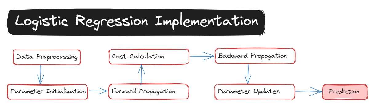
• Here is the summary image of the implementation:

Importing the Packages

import numpy as np 
import matplotlib.pyplot as plt
from sklearn import datasets
from sklearn.model_selection import train_test_split
import requests
from PIL import Image
from io import BytesIO

• We are using the numpy module to work with scientific calculations as well as matrix operations, which we will see soon.

• We are using matplotlib to plot the image as well as the graph and it is quite useful for data visualization.

• We are using sklearn datasets, to import the MNIST dataset from the library directly instead of downloading it from the website.

• We are importing train_test_split from the sklearn model selection, so that we can split the data into train data and test data, so that we can train the model using the training data and test it by making predictions on the test data.

• We are requesting a module to get the images from the internet to test the model.

• We are PIL (Python Imaging Library) so that we can make some operations on the images that we take from the internet.

• We are using the BytesIO module so that we can temporarily store the image, which is taken from the internet, instead of downloading the image into the local disk.

Importing the Data

digits = datasets.load_digits()
print(digits)
print(digits.images.shape)  # Will show (1797, 8, 8)
print(digits.images[0])  # Prints the first 8×8 image
print(digits.data.shape) # (number of training examples, 64) As it is a 1D array there will be 64 columns per image.
idx = np.where((digits.target == 0) | (digits.target == 1))[0]
print(idx)

• We can see that there are 1797 images in the dataset.

• When you print digits, they will appear as images flattened into a 2D array. Each row has 64 numbers (representing the 8×8 pixel values stretched into a line). The values range from 0 to 16, where 0 is white and 16 is black.

• By printing the first image from the digits, you can see the 2d array of the image(8×8).

• By printing the shape of the data in digits, we can see that there are 1797 training examples and each example is an array of length 64.

• The idx will print the indexes of the images that contain either 1 or 0 as the value.

Plotting the image

# you can take the above indexes and place it here you can either see a 1 in the plot or 0.
import matplotlib.pyplot as plt
from sklearn import datasets

# Load the digits dataset
digits = datasets.load_digits()

# Display digit at index 0
plt.figure(figsize=(4, 4))
plt.imshow(digits.images[861], cmap='gray') # change the index so that you can change image of the number and .images[] get the 3d array of the image
plt.title(f"This is a {digits.target[861]}") # change the index so that you can change the label of the number
plt.axis('off')
plt.show()# you can see it is a 8 * 8 image which means there are maximum 16 pixels (0 to 16)
# 0 represents white/blank space
# 16 represents the darkest shade (black)

• Here we use matplotlib to visualize the image of the number with index 861. This index contains a value of 1, so you can visualize the image of 1.

• If you comment out the plt.axis(‘off‘) you can see the grid which shows till 7 horizontally and 6 vertically that means this is an 8 × 8 image.

Loading the dataset

def load_basic_dataset():

    # Load digits dataset from sklearn
    digits = datasets.load_digits()

    # We'll use only digit 0 and 1 to make it a binary classification like cat/non-cat
    idx = np.where((digits.target == 0) | (digits.target == 1))[0]
    X = digits.data[idx] # this will get the 2d array of the image
    y = digits.target[idx] # gets 1d array from 0 to 9, but we will only get either 0 or 1 because idx's are the indexes of 1's and 0's

    # Split dataset into train and test sets
    X_train, X_test, y_train, y_test = train_test_split(X, y, test_size=0.2, random_state=42)

    # Reshape to the format (features, examples)
    X_train = X_train.T / 16.0  # Normalize to [0,1] - maximum value of a pixel in MNIST is 16
    X_test = X_test.T / 16.0
    y_train = y_train.reshape(1, -1)
    y_test = y_test.reshape(1, -1)

    classes = np.array(["non-digit-1", "digit-1"])

    return X_train, y_train, X_test, y_test, classes

• We are going to load the MNIST dataset from the sklearn instead of downloading it into the local disk.

• You can see we used idx here, which we printed in the previous code, so that it acts like a threshold for the indexes and takes only those as the input for X and y instead of the whole dataset.

  Why? Because we need to classify whether the digit is 1 or not. So we only use two values in the dataset 0 and 1.

• We are normalizing the data in the 7th line by dividing the data by 16.

  What is Normalization, and why do we do it? Normalization is the process of standardizing the scale of the data. We do this process so that while doing the training, the data converges faster compared to without normalization.

• In this script, we are dealing with the MNIST dataset, based on this dataset, I am dividing it by 16 because it will normalize the scale of the data to [0,1].

• Then we initialize two classes, one is non-digit-1 and the other is digit-1.

• Using this function, we are splitting the data into train and test data as well as we are initializing the classes, which can be used as y(true outputs) for the model to classify the data into these classes.

Sigmoid Function

# We have divided the data into train and test data.
# Now as we know in logistic regression we wont take the data directly, we will apply sigmoid function as it is a classifcation model
# We need to make sure solution will be between 0 and 1 instead of 0 to infinity, so that's the reason we apply sigmoid function 
# We all know the formula of sigmoid function is 1/(1+e^-x). 
# So let's make the code to  sigmoid funciton
def sigmoid(z):
    """
    Compute the sigmoid of z

    Arguments:
    z -- A scalar or numpy array of any size.

    Return:
    s -- sigmoid(z)
    """
    s = 1 / (1 + np.exp(-z))
    return s

Before explaining the code, I will ask you a question?

What is a sigmoid function?

• Sigmoid function is an S-shaped mathematical function used commonly in Machine learning.
• This function will output a value between 0 and 1
• It helps the model to learn non-linear relationships
• In Logistic regression it will convert the linear combination of features into probability.
• This is useful for binary classification.

Here is the formula for the sigmoid function -:

$$\sigma(x) = \frac{1}{1 + e^{-x}}$$

• We just implemented this formula as the function in the above code.

Why do we use the exponential value instead of numbers like 2, 4, or 100? While it's true that we could replace e with any other value greater than 1 and still retain the S-curve shape, the graph would either stretch or compress depending on the value chosen, adding unnecessary complexity. One key reason for using e is related to the derivative of the sigmoid function. If we replace e with a variable k, the derivative becomes s(x) \ (1 - s(x)) * ln(k). To eliminate the ln(k) term and simplify calculations, particularly in backpropagation and also in deep learning neural networks, we set k to e. This choice ensures mathematical efficiency and consistency.*

We are creating this function because, in logistic regression, one of the initial steps involves applying the sigmoid function to the data.

We know that we use y = wx + b for the logistic regression implementation that outputs the value from (-infinity to +infinity). To obtain binary output for logistic regression, we classify the result of the linear combination. Outputs closer to zero are categorized as 0, while those closer to one are categorized as 1. Here, a prediction of 1 indicates "digit-1" whereas a prediction of 0 signifies "not-digit-1" . This is the essence of how the sigmoid function operates. Observing its graph can provide additional clarity. Below is the sigmoid function's graph for reference.

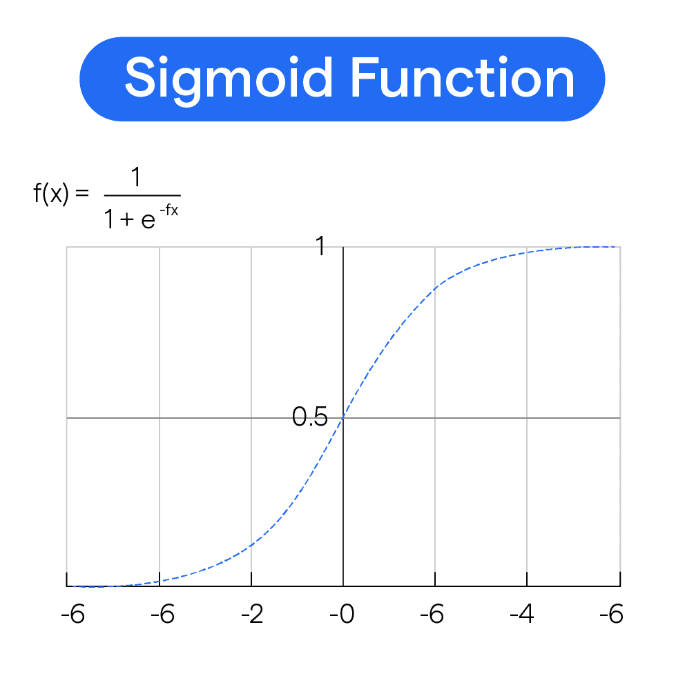
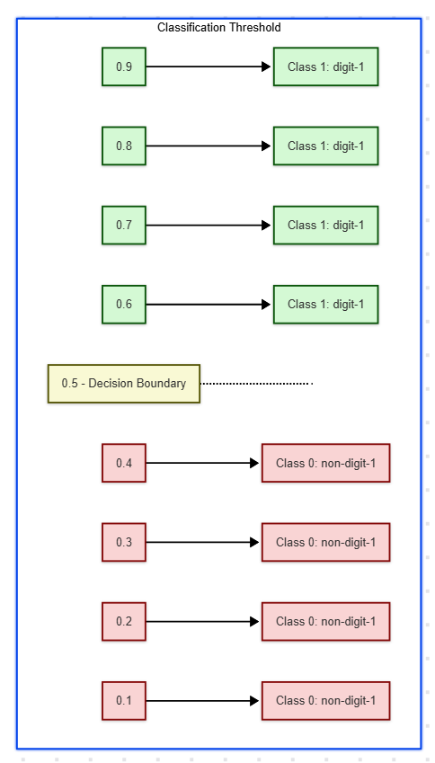
If the value exceeds the threshold of 0.5, it is considered positive, while a value below 0.5 is deemed negative. In practice, the selection of the threshold may vary depending on the specific problem.

The code utilizes the numpy function np.exp() , which is specifically designed to handle vectors and arrays. While the math module provides a similar function, math.exp() it is limited to working with single values and is therefore unsuitable for machine learning tasks that require operations on arrays or matrices. The numpy function np.exp() effectively addresses this limitation.

Initializing parameters

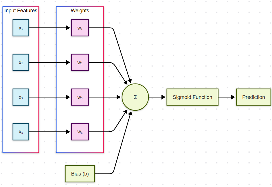
We will initialize the weights(w1,w2,..wn) and bias(b) to apply sigmoid function and get the prediction.

def initialize_with_zeros(dim):
    """
    This function creates a vector of zeros of shape (dim, 1) for w and initializes b to 0.

    Argument:
    dim -- size of the w vector we want (or number of parameters in this case)

    Returns:
    w -- initialized vector of shape (dim, 1)
    b -- initialized scalar (corresponds to the bias) of type float
    """
    w = np.zeros((dim, 1))
    b = 0.0

    return w, b

• There are two parameters that we use in logistic regression, those are:

  • weights(W or w)

  • bias(b)

• We are introducing these two parameters to enhance the model's learning process.

• During model training, we use two key parameters as variable values. Other parameters include cost and loss. To ensure the loss parameter is minimized, we need to update the two critical parameters, w and b.

• In the above code we are initializing the values of W and b to 0.

Maybe you guys have some questions right now like:

Why am I representing weight as both w and W?

I am representing them as w or W, there is a difference between them, w → scalar value, and W → vector consisting of multiple weights.

Why am I initializing the value of W and b to 0?

That’s a great question! In logistic regression, we typically initialize the parameters to zero for simplicity, as it works well with the convex cost function. However, this approach doesn’t apply to neural networks. While we could initialize the values of w and b to 1 or any other value, doing so would impact the number of iterations required for convergence.

• We are initializing the shape of the matrix W to (dim,1). Here dim is the value of 64, the dimension of a single image.

• The code utilizes the NumPy function np.zeros() , which is ideal for generating a matrix of specified dimensions, completely filled with zeros.

Forward and Backward propagation

Now that your parameters are initialized, you can do the "forward" and "backward" propagation steps for learning the parameters.

propagate

The above code is implementing a function propagate() that computes the cost function and its gradient.

Hints:

Forward Propagation:

• You get X

• You compute

$$A = \sigma(w^T X + b) = (a^{(1)}, a^{(2)}, ..., a^{(m-1)}, a^{(m)})$$

• You calculate the cost function:

$$J = -\frac{1}{m}\sum_{i=1}^{m}(y^{(i)}\log(a^{(i)})+(1-y^{(i)})\log(1-a^{(i)}))$$

• Here are the two formulas you will be using for backward propagation:

$$\frac{\partial J}{\partial w} = \frac{1}{m}X(A-Y)^T$$

$$\frac{\partial J}{\partial b} = \frac{1}{m} \sum_{i=1}^m (a^{(i)}-y^{(i)})$$

Here is the code to implement these formulas:

def propagate(w, b, X, Y):

    m = X.shape[1] # number of training examples we are using for the problem that means number of images(2d arrays)

    # Forward propagation
    Z = np.dot(w.T, X) + b
    A = sigmoid(Z)

    # Add epsilon to avoid log(0)
    epsilon = 1e-10
    cost = -np.sum(Y * np.log(A + epsilon) + (1 - Y) * np.log(1 - A + epsilon)) / m # dividing by m to get the average cost

    # Backward propagation
    dw = np.dot(X, (A - Y).T) / m # dividing by m to get the average gradient
    db = np.sum(A - Y) / m

    cost = float(np.squeeze(cost))

    grads = {"dw": dw, # change in weight and change in bias
             "db": db}

    return grads, cost

• We are developing a function called propagate(), which takes the arguments w, b, X, and Y, whose purposes are already familiar to you.

• This function will return the gradient values(dw,db) and the cost value.

• We are initializing a value inside this function, ‘m’ which is the number of training examples.

• We are going to find the value of Z that will be useful to find the activation value using the variable ‘A’.

• Then we are going to find the value of cost using the cost function that utilizes the value of A and Y.

• np.squeeze() converted the unnecessary array into a numerical value. float() will convert the data type of that value into a float.

• We will return the grads and cost using this function.

• These two parameters then can be used to optimize the values of w and b.

• Maybe you will get a question like,

  Why are we finding gradients dw, db? These are useful to optimize the values of w and b in the optimize() function that we can discuss in the next part.

  Why didn’t we implement a variable loss function which we learnt in the previous blog, as maximum likelihood? So while we didn't explicitly mention maximum likelihood in the code, the binary cross-entropy cost function we're using is mathematically equivalent to maximizing the likelihood of our observed data under a Bernoulli probability model.

Maximum Likelihood Formula -:

$$\text{Likelihood function: } L(w,b) = \prod_{i=1}^{m} p(y^{(i)}|x^{(i)};w,b)$$

$$\prod_{i=1}^{m} p(y^{(i)}|x^{(i)};w,b) = \prod_{i=1}^{m} (h_\theta(x^{(i)}))^{y^{(i)}} (1-h_\theta(x^{(i)}))^{1-y^{(i)}}$$

$$\text{Log-likelihood: } \log L(w,b) = \sum_{i=1}^{m} y^{(i)} \log(h_\theta(x^{(i)})) + (1-y^{(i)}) \log(1-h_\theta(x^{(i)}))$$

$$\text{Negative log-likelihood: } -\log L(w,b) = -\sum_{i=1}^{m} \left[ y^{(i)} \log(h_\theta(x^{(i)})) + (1-y^{(i)}) \log(1-h_\theta(x^{(i)})) \right]$$

We use negative log-likelihood because, during model development, optimization algorithms are typically designed to minimize rather than maximize. We take the average of the above function to get the cost function of the logistic regression which can be act as the loss function also.

$$\text{Cost function: } J(w,b) = -\frac{1}{m} \sum_{i=1}^{m} \left[ y^{(i)} \log(h_\theta(x^{(i)})) + (1-y^{(i)}) \log(1-h_\theta(x^{(i)})) \right]$$

Conclusion

So far, I have discussed several functions that are essential for developing a logistic model and making predictions. This is Part 1 of the series. In the next part, I will demonstrate how to utilize these functions, along with additional ones, to build the logistic model and perform classification tasks.

To summarize the blog, developing a logistic model involves two key functions: the cost function and the loss function. To implement these, additional components like the sigmoid function, linear combination of input and parameters(Z), and the Activation Function(A) are required. Two essential parameters, weights (W) and bias (b), are initialized with random values. By the end of the model's development, these parameters are optimized to achieve their best possible values, ensuring the loss is minimized.

Action Step:

Try tracking these calculations for a few iterations with a different tiny image, like:

[16 0]
[16 0]

This could represent a vertical line on the left.

With label y = 0 (not a digit 1), follow the same steps and see how the model learns to classify it correctly.

Implement the functions which I explained you in this blog and practice them

You can practice the concept on paper.

References

These are the references that will be helpful to get to know more about this concept:

1. Here is the code: https://github.com/Dhyuthidhar2404/personal_blog/blob/main/Logistic_Practice.ipynb

2. Deep Learning or Machine Learning course by Andrew Ng in Coursera.

3. The 100 Pages of ML book by Andriy Burkov

4. Introduction to logistic regression blog

These two are wonderful resources to learn these concepts.

Why I Share This

Simon Squibb believes that the best way to share knowledge is to make it simple and accessible. That’s exactly what I do—I break down complex technology into something easy and exciting.

Tech should inspire you, not intimidate you.

Imagine a world without machine learning—every company would need to manually analyze massive datasets just to extract insights. Deep learning changed that game. It enables anyone with data to uncover patterns and build intelligent systems without relying solely on traditional methods.

I share knowledge this way because I want you to feel that excitement too.

If this post made you think differently about tech, check out my other blogs. Let’s make tech easy and exciting—together! 🚀